SUPRI-D Research Projects
A NEW LOOK INTO NONLINEAR REGRESSION
Aysegul Dastan, PhD candidate
Nonlinear regression has long been used to fit reservoir models to well test data for the estimation of reservoir parameters. In many cases the estimation strategy and the choice of the estimation parameters make a difference. Considering a simple model with wellbore storage and skin, the parameters to be estimated are permeability (k), wellbore storage coefficient (C), and skin factor (s). In a least-squares estimation strategy, such as Gauss-Newton, the estimation parameters could be chosen as [k, C, s]. This choice makes an implicit assumption as to the distribution of these parameters, which may not reflect their actual distribution. A better search strategy and more accurate estimations may be obtained if the probability distributions of these parameters can be incorporated in the estimation process.
Positive parameters that are associated with a probability density f(x)=a/x are called Jeffrey’s parameters (Tarantola 2005). In nonlinear regression it is argued that a Cartesian conversion can help the estimation process. Using the natural logarithm of a Jeffrey’s parameter results in a Cartesian parameter, in that the parameter has a homogeneous distribution. For example using log(k) instead of k is probably advantageous since k has lognormal probability distribution in nature. To examine the possible advantages of using different parameters, we developed a nonlinear regression program in MATLAB. This program can incorporate a variety of reservoir models such as wellbore storage, skin, and dual porosity. The program can also use convolution to incorporate the rate history, for example, a series of drawdowns and build-ups. It has a standardized input file format so that these preferences and the pressure history data can be entered. We generalized the idea of Jeffrey’s parameters vs. Cartesian parameters and designed the program to be able to try any functional form for the parameters to be estimated. For a simple drawdown, for example, instead of making the iterations on the Jeffrey's parameters [k, C, s] we can use the approximately Cartesian parameters [log(k), log(C), log(s+8)]. Using different functional forms may have an effect on the final converged result and on the number of iterations to achieve that.
So far, on simple problems we have not found a significant advantage of using Cartesian parameters over Jeffrey’s parameters. We can see that the iterations starting from the same initial point follow a different path to reach the final converged result. Table 1 shows the iteration results for the case with Jeffrey’s parameters, i.e. using the parameters [k, C, s] for a drawdown experiment, while Table 2 shows the path when Cartesian parameters [log(k), C, s] are used.
Table 1: Iterative sequence using k, C and s as solution paramers.
iteration |
k (md) |
C (STB/psi) |
s |
Error |
0 |
150 |
0.01 |
5 |
5775750.5994 |
1 |
111.0491 |
0.014887 |
3.4818 |
444932.9073 |
2 |
146.224 |
0.016364 |
6.2979 |
17868.7046 |
3 |
161.301 |
0.016386 |
7.5413 |
240.4242 |
4 |
162.9871 |
0.016384 |
7.6832 |
116.176 |
5 |
163.0043 |
0.016384 |
7.6847 |
116.169 |
Time elapsed: |
14.031 s |
|
|
|
Table 2: Iterative path using [log(k), C, s] as solution parameters.
iteration |
k (md) |
C (STB/psi) |
s |
Error |
0 |
150 |
0.01 |
5 |
5775750.5994 |
1 |
115.6956 |
0.014887 |
3.4818 |
154384.9236 |
2 |
153.441 |
0.016432 |
6.3637 |
462711.609 |
3 |
162.5179 |
0.016399 |
7.5907 |
4671.5987 |
4 |
163.0009 |
0.016384 |
7.6841 |
116.2504 |
5 |
163.0043 |
0.016384 |
7.6847 |
116.169 |
Time elapsed: |
14.422 s |
|
|
|
For the initial runs with a limited number of data sets, we did not observe a significant performance difference between the use of Jeffrey’s parameters or Cartesian parameters. Both of these tests gave the same fit for the data, as shown in Figure 1.

Figure 1: Fits to the data, after the iterative sequences shown in Tables 1 and 2.
Figure 2 shows a fit for another data set. This time a reservoir model with dual porosity was used.
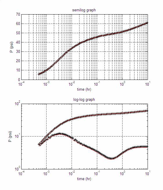
Figure 2: Fits to the data, in a dual porosity case.
We did not observe a performance difference between using Cartesian and Jeffrey’s parameters in the dual porosity case either. However, by using different initial estimates and different data sets, we expect that using Cartesian parameters will be advantageous. In addition, modeling more complex tests (such as a set of consecutive drawdowns and buildups) may be more sensitive to the choice of parameters. There are other tests where there is ambiguity in interpretation due to small number of data points, where it may also be possible to see performance.
The conclusions we will draw from this study will help better understand the reservoir models that we currently use and obtain more robust parameter estimation techniques. This will enable reservoir engineers to predict future reservoir behavior more reliably.
References
Tarantola, Albert Inverse Problem Theory and Model Parameter Estimation, SIAM, 2005. [http://www.ipgp.jussieu.fr/~tarantola/Files/Professional/Books/index.html]