Projects

A NEW LOOK INTO NONLINEAR REGRESSION

Aysegul Dastan, PhD candidate

Well testing provides a set of useful tools to estimate reservoir parameters.  Based on the estimates, it is possible to forecast the reservoir behavior for future production and hence a reservoir can be utilized in an optimal way.  Nonlinear regression was introduced to well testing more than two decades ago and revolutionized well testing with new methods and substantially improved the accuracy of the prediction.  However, limited improvement has been achieved for some time.  In our work we take a new look at nonlinear regression in well testing and develop novel methods to improve its accuracy and prediction capability for a variety of well test data.

• Inverse Problems in Well Testing

In well testing we consider the reservoir as a black box that has an input and an observable output.  Through physical laws, the input and the output can be related mathematically in terms of a set of unknown parameters.  Inverse problem solving is the process of inferring the unknown parameters using this mathematical relation and input-output data.

In most cases, the pressure transient observed at a well is the observable output and the injection/production rates are the inputs.  Using physical laws, a mathematical relation can be found between pressure transient and injection rate.  Let us assume the pressure transient can be represented by the function f.  This function depends on the parameter set a, which is a vector of the form , and the time variable t: .  This function could, for example, be the pressure response of a drawdown test, for which the input is a unit-step function (i.e., the production is zero before t=0 and it is at a constant rate q0 for t>0).  In well testing, our goal is to estimate the unknown parameter set a given a pressure transient data p(t).  Such problems, where actual measurements are used to infer the values of system parameters are called inverse problems.  The ‘forward’ problem, on the other hand, corresponds to the mathematical modeling of the system.
 
The general recipe for the analysis of a physical system (in our case, the reservoir) can be divided into three steps: (Tarantola, 2005)

1. Parameterization of the system: A minimal set of model parameters is determined such that the system, from a given point of view, is characterized completely.
2. Forward modeling: Relating the model parameters through physical laws to make predictions on some observable parameters.
3. Inverse modeling: Using actual measurements of observable parameters to infer the actual values of model parameters.

My research concentrates on the third step, inverse modeling.  We have investigated the impact of making transformations on the parameter space and on the data space.

• Transformations on the parameter space:

In nonlinear regression it is possible to use a transformed parameter space a*, which is a function of a.  As an example, the logarithm of permeability has been used in some applications for parameter estimation and it is known to improve the performance in general.  The reason behind this, however, is more generally instructive. 

In a nonlinear regression problem, the parameters that are estimated are tacitly assumed to be Cartesian.  In other words, when searching for a solution for the permeability, for example, we assume (in the absence of any other information) that the probability of finding the solution is uniformly distributed in the Cartesian coordinate space, such that the probability distribution function is , where k is a constant.  This, however, may not be the case for many physical parameters.  There is another class of parameters that have probability distribution .  These are called Jeffreys parameters.  It can be shown that taking logarithms of Jeffreys parameters results in Cartesian parameters.  Consequently, taking the logarithm of permeability allows us to use a Cartesian parameter in the estimation.  In addition to permeability, other well test parameters can also be assumed to be Jeffreys parameters and various transformations can be applied to obtain a Cartesian parameter set for nonlinear regression.

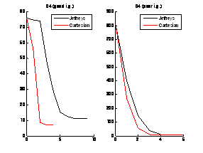
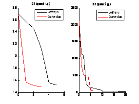
In the following test, we compared using Jeffrey’s parameters and Cartesian parameters (the transformed parameter space).  We observed that if good transformations can be found to give Cartesian parameters, the performance of nonlinear regression is enhanced.
 

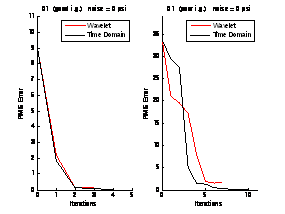
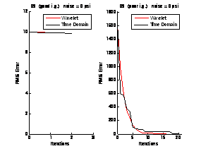
In these graphs, the x axis shows the number of iterations and the y axis shows the error (objective) function.

• Transformations on the data space:

In addition to making transformations on the parameter set we are also investigating transforming the data set itself.  With such a transformation, it is possible to realize certain operations, including compressing and denoising the data.  Thus far we have explored the wavelet transform, which is a convenient way of handling long data sets with many data points. 

In our technique, we use a limited number of wavelet coefficients to represent the data and use the nonlinear regression algorithm on this transformed data to estimate the parameters.  This process not only compresses the data (without deleting hard data points) but also eliminates the noise.  We are considering a number of strategies to choose a given number of wavelet coefficients.  We have tried choosing based on the magnitude of the wavelet coefficients only.  It is also possible to make some kind of sensitivity analysis to determine which wavelets should be chosen.  We observed that with only a few wavelet coefficients it is possible to achieve the same converged result as using the untransformed data.  In the examples that follow, we used seven wavelet coefficients to represent the function and made the fits on these seven coefficients at each iteration.  These iterations are compared to the case where the fits are made on the actual complete pressure data points rather than the wavelet transform.  We see that with the wavelet transform, we obtain comparable performance in many cases, and in some cases the wavelet transform process outperforms the analysis of the full data set.

In addition to the wavelet transform, we are also working on methods that fit pressure derivatives rather than the pressure data.  Methods based on the pressure derivative are expected to be more robust especially for dual porosity reservoirs.

• Conclusion

In conclusion we are developing nonlinear regression algorithms that are faster, and more robust to poor initial guesses.  Moreover we provide an approach useful for application to massive data sets from permanent downhole gauges.  Finally, we are also developing algorithms with inherent noise removal properties.

References
Mallat, S., 1999, “A wavelet tour of signal processing,” 2nd Ed. Academic Press
Tarantola, Albert  Inverse Problem Theory and Model Parameter Estimation, SIAM, 2005. [http://www.ipgp.jussieu.fr/~tarantola/Files/Professional/Books/index.html]